KuboLog 2008-01-25

2008 年 01 月 25 日 (金)

0840 起床．ねむいよー …… 0900 自宅発．晴． 0920 研究室着．コーヒー．朝飯．

昨日からサケ + アミノ酸文献とかぽつぽつとながめてるんだが …… サケが「ここを溯上しよう」って決定するのはホントに河川水中のアミノ酸組成がカギになってるのかしらん? いや，なんだかハナシがもうそういう方向で広まりつつあるのは知ってますよ (少なくとも国内では) ……

サケの嗅覚がアミノ酸に応答しうる，という神経生理学的な研究には特に異論はないんだけど (というかそれほどちゃんと論文よんでないんだけど)， Y 字型人工水路を使った選択実験ってこれでいいのかしらん? 原著論文として出ているものは (おそらく) ひとつだけで (2003 年)，天然状態の湖水が流れる水路とアミノ酸とか人工的に調整した水 (詳細不明の味の素社による特製もの) を流した水路で比較すると味の素の水のほうを選んだ魚が多かった，というだけだよね．日本語で書かれた解説によると他にもいろいろ実験してたみたいなんだけど (この中には「複数の味の素の水を流した場合」という私が知りたい状況なんかも含まれているようだけど)， 2003 年以降はこの実験に関する論文はまったく出ていない．

他にも「鼻に栓」実験とかもあるらしいんだけど (上記解説文にはこれについては書いてないけど)，これまた文献がみあたらない ……

で，上記解説文では味の素の水の何が重要だろうかを調べるハナシ (論文なし) が紹介されてて，グルタミン酸 (Glu) が一番おおいから (ちなみにてもとの天塩川データでは Glu は多くない)， Glu を除去してみたところ …… という実験やっても Glu ぬきを嫌ってなかったみたいだから，単一アミノ酸の多い少ないではなくて複数アミノ酸のぶれんど具合が重要かもねといったハナシになっている．おそらくこのへんの流れから，今の院生たちがあちこちの川で水をくんできてアミノ酸組成を調べることになってるんだよね．

で，ふつーの河川中のアミノ酸組成なるものは，データを見ればわかるように場所・季節によってばんばん変わるもの．そしてアミノ酸組成測定なんて現代ではもはや簡単だろう，といった憶測とはうらはらになかなか正確には測定できないもの，のように見えるんだよねえ …… まあ，この点に関してはサケの嗅覚器管にだって個体差なんかもあるんだろうし，人間が取得した観測値にノイズが多くても騒ぐほどではないかもしれぬ．

よくわからんのは，たくさんあるうちの 2-3 個のアミノ酸の組み合わせが重要かも，といったハナシ．たとえば A と B といったアミノ酸の組み合わせが重要だとして， (例によって「割算」思考で) A 対 B の比がある値に保たれていれば OK みたいなハナシ，があったとしよう …… 昨日からいろいろ考えているんだけど， A や B の絶対濃度に関係なくその比 (すなわち対数の差) がある範囲にある場合にだけ応答する，というニューラルネットは簡単には構成できないように思うんだよねえ．

いやもちろん下の図ぐらいのにゅうらるねっと (これはどちらかといえば複雑というより単純な部類だと思うんだが)，「学習」とやらを適切にやればパターン識別なんかは簡単にできるわけだけどね．

[アリ個体にゅうらるねっと]

ぎょーむ日誌 2007-07-25 より …… library(MASS) の nnet() で生成された人工にゅうらるねっとの例．実データを正規乱数で修飾した炭化水素 (人工) データ 200 パターンでトレイニングされたあるにゅうらるねっとアリ個体．上から出力層・隠れ層・入力層．入力層は 25 個のけみかる感覚素子からなっている．赤い結線はプラス，青い結線はマイナスの加重，太さは加重の大きさをあらわす (加重がゼロにちかい結線は描画してない)．入力層・隠れ層の数値は閾値．

てなこと書いてると，アミノ酸データとった Nina さんからメイルがきたので返信かき．次々と対応策を考えてくれて，なかなかすばらしい．

ともあれ，いきなりにゅーらるねっととかやったらワケわかんないことになるのは必定なので，ともかく作図・作図 ……

今回は pairs() を工夫してみた．二変量正規分布 (二次元正規分布; bivariate normal distribution) の confidential region (信頼領域?) は library(ellipse) ( R Graphical Manuals の図) の ellipse() 関数を使って描画．

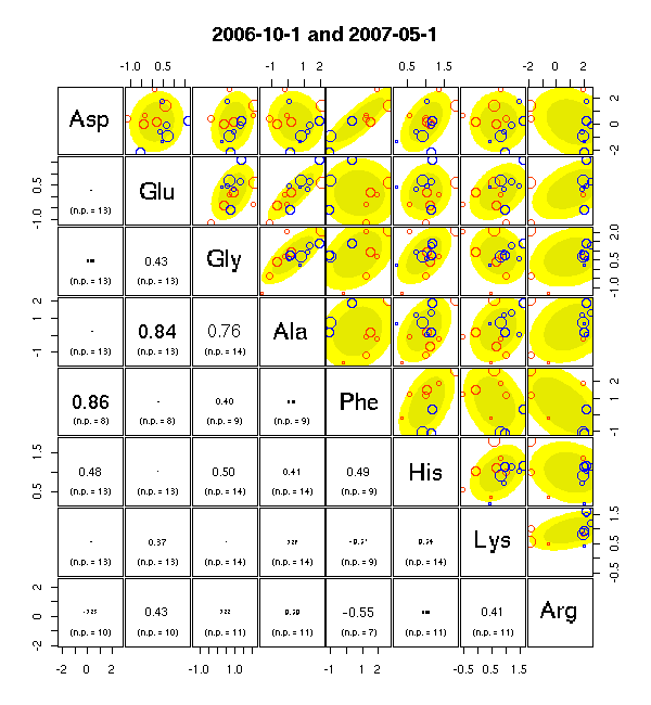
pairs(..., upper.panel = pfunc1, ...) の pfunc1 パネル関数はこんなかんぢで．

plot.ellipse <- function(x, y, level, col)
{
	f <- is.finite(x) & is.finite(y)
	x <- x[f]
	y <- y[f]
	exy <- ellipse(cor(x, y), level = level)
	polygon(
		mean(x) + exy[,1] * sd(x),
		mean(y) + exy[,2] * sd(y),
		border = NA,
		col = col
	)
}

pfunc1 <- function(x, y)
{
	plot.ellipse(x, y, 0.8, col = "#ffff00")
	plot.ellipse(x, y, 0.5, col = "#eeee00")
	points(
		x, y,
		col = c(rep("#ff4000", n.location), rep("#0000ff", n.location)),
		pch = 21,
		cex = v.col * 0.25
	)
	usr <- par("usr"); on.exit(par(usr))
	par(usr = c(0, 1, 0, 1))
	rect(0, 0, 1, 1)
}

で，また Nina さんにメイル書き，と．これでしばらくこちらの下うけは休止してよいだろう．

で，リモートが終了したらローカルな下うけ，ということで稲葉さんと石狩浜ハマエンドウ花芽数の library(VGAM) な vglm() 解析にとりくんでみる．これの family = posnegbinomial すなわち positive negative binomial 分布なる positive なのか negative なのかはっきりしてくれーな分布 (その実体はゼロが「見えない」負の二項分布) なるモノがつかえるのだけど …… これも glm.nb() と同じくデータ数が少ないときは計算を途中で投げ出してしまう，とわかった．おとなしく family = pospoisson とする …… 実際のところ，ちょっと overdispersion ぎみな気もするんだが．

旅費書類かきとかすませて， 1950 研究室発．雪． 2005 帰宅．体重 70.2 kg．お，いきなり 1kg おちた．ちょっとうんどう．晩飯．

[今日の運動]

腹筋運動 30 × 3 回．腕立ふせ 10 × 3 回．スクワット 100 回．

[今日の食卓]

朝 (0940): 研究室．食パン．
昼 (1330): 研究室．食パン．
晩 (2200): 米麦 0.8 合．卵焼き．ハクサイ・ダイコンのコンソメスープ．

ぎょーむ日誌 2008-01-25

2008 年 01 月 25 日 (金)